Model 2a Mixing of LFR and CSP Outlet Streams

In Model 2a we independently call the collector_receiver and nuclear_plant to determine some outlet temperature and mass flow for each. Before entering the hot salt tank, the two streams must mix together.

Outlet Temperature Differences

Problems could arise if the outlet temperatures from each plant differ by too much. Here is a plot of the temperature differences between the two outlet temperatures:

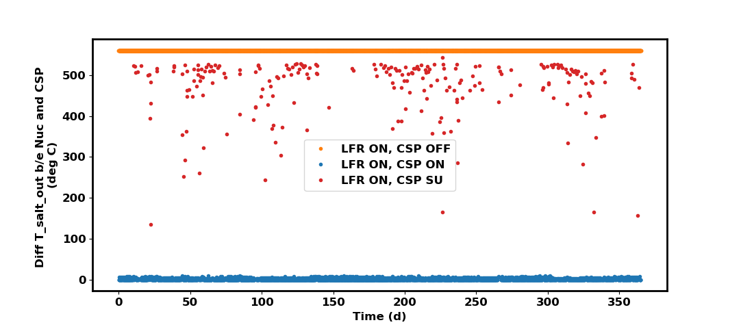
Note that the nuclear_plant conditions are just calculated in SSC, they are not applied to the actual model yet in this case. Three major categories exist for the temperature differences:

• LFR is ON and CSP is OFF: the collector_receiver in this case returns a 0 temperature which the TES solver would normally convert to the previous temperature of the hot salt tank. The mass flow is also 0 when the CSP plant is OFF. The nuclear_plant does return an outlet temperature and mass flow (hence the \(560^\circ C\) temperature difference corresponding to the desired hot tank temperature). We can use this as the input to the TES for this particular scenario.

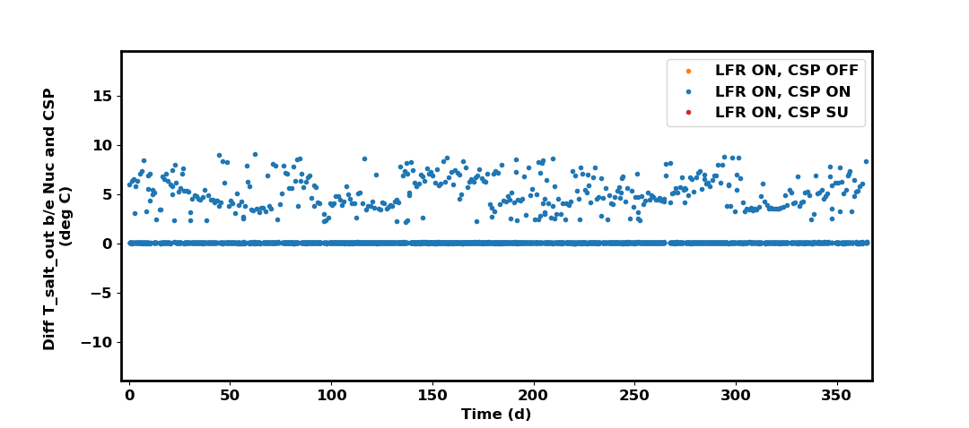
• LFR and CSP are both ON: both the collector_receiver and nuclear_plant return an outlet temperature and mass flow. From the figure, you can see that the outlet temperature differences are small, at most a difference of \(10^\circ C\). Therefore, some sort of mixing should happen before incorporating both streams as a TES input.

• LFR is ON and CSP is in STARTUP: here there are bigger disparities in outlet temperature due to the CSP startup mode. Stream mixing is more important here, we should take care to apply proper enthalpy balance.

Enthalpy-Averaged Mixing

Ultimately, the mass flow of the mixture will be

\[\dot{m}_{mix}^H = \dot{m}_{nuc}^H + \dot{m}_{rec}^H\]

given the nuclear_plant and collector_receiver outlet conditions, where the superscript \({}^H\) represents the hot outlet node before entering the hot storage tank.

We can then find the final temperature of the mixture first through enthalpy balance and then converting back to a temperature. First we need a formula that converts the temperature of the molten salt to its enthalpy:

\[h_{salt}^N = f(T_{salt}^N)\]

where the superscript \({}^N\) can represent either \({}^H\) from before or \({}^C\), the cold inlet node just after leaving the cold storage tank.

We then find the enthalpy change across each respective plant as

\[\Delta h_{plant} \equiv h_{salt}^H - h_{salt}^C.\]

The enthalpy of the combined outlet stream is then calculated from the first law of thermodynamics

\[\Delta h_{mix} = \frac{\dot{m}_{nuc}^H \Delta h_{nuc} + \dot{m}_{rec}^H \Delta h_{rec}}{\dot{m}_{mix}^H} \equiv \bar{h}\]

Note that \(\bar{h}\) is dependent on solved properties of the flow at each plant’s outlet temperature.

Available SSC HTF Properties

For the temperature-to-enthalpy conversion, we need to know the specific heat of the heat transfer fluid (HTF). SSC has a dedicated HTFProperties class with conversions between different thermodynamic properties. Note that our specific molten salt is \(60 \% \ \text{NaNO}_3, \ 40\% \ \text{KNO}_3\). An empirical relation between temperature and specific heat is given:

\[C_p(T) = a_1 T^3 + a_2 T^2 + a_3 T + a_4\]

where

\[\begin{split}\begin{align} a_1 &= -1\times 10^{-10} \frac{kJ}{kg \cdot K^4} \\ a_2 &= 2\times 10^{-7} \frac{kJ}{kg \cdot K^3} \\ a_3 &= 5\times 10^{-6} \frac{kJ}{kg \cdot K^2} \\ a_4 &= 1.4387 \frac{kJ}{kg \cdot K}. \end{align}\end{split}\]

There exist conversions from temperature to enthalpy and vice-versa, however these are just for nitrate salts and not for the potassium nitrate mixture.

Converting Temperature to Enthalpy

Because the specific heat is neither constant nor linear, we need a more complex derivation for the enthalpy as a function of temperature. We begin with the definition of specific heat:

\[C_p(T) = \frac{dh}{dT} \bigg|_{P=\text{constant}}\]

We can then set

\[\frac{dh}{dT} = a_1 T^3 + a_2 T^2 + a_3 T + a_4\]

and integrate both sides from \(T_{salt}^C\) to \(T_{salt}^H\)

\[h_{salt}^H - h_{salt}^C = \int^{T_{salt}^H}_{T_{salt}^C} a_1 T^3 + a_2 T^2 + a_3 T + a_4.\]

If we define a formula

\[h_i (T) = \frac{a_1}{4} T^4 + \frac{a_2}{3} T^3 + \frac{a_3}{2} T^2 + a_4 T\]

then we can combine with the previous equation:

\[\Delta h_{plant} = h_{salt}^H - h_{salt}^C = h_i(T_{salt}^H) - h_i(T_{salt}^C).\]

We can apply the above equation to both the nuclear_plant and collector_receiver with their respective solved outlet conditions.

Converting Enthalpy to Temperature

Now that we have a relationship between enthalpy and temperature, we can write that

\[\Delta h_{mix} = h_i(T_{mix}^H) - h_i(T_{mix}^C) = \bar{h}\]

and, assuming that \(T_{mix}^C = T_{salt}^C\) (which we assume is the same for both plants), solve for the hot outlet temperature for the mixture:

\[h_i(T_{mix}^H) = \bar{h} + h_i(T_{salt}^C) = \frac{a_1}{4} ({T_{mix}^H})^4 + \frac{a_2}{3} ({T_{mix}^H})^3 + \frac{a_3}{2} ({T_{mix}^H})^2 + a_4 ({T_{mix}^H}).\]

To find \({T_{mix}^H}\) we need to solve a quartic equation

\[Ax^4 + Bx^3 + Cx^2 + Dx + E = 0\]

where

\[\begin{split}\begin{align} A &= \frac{a_1}{4} \\ B &= \frac{a_2}{3} \\ C &= \frac{a_3}{2} \\ D &= a_4 \\ E &= -(\bar{h} + h_i(T_{salt}^C)) \end{align}\end{split}\]

which are all known values at this stage and \(x\) is \({T_{mix}^H}\). We can solve this according to the initial method proposed in Strobach (2010), where we recast the coefficients as

\[x^4 + ax^3 + bx^2 + cx + d = 0\]

with

\[\begin{split}\begin{align} a = \frac{B}{A} &, \ b = \frac{C}{A} \\ c = \frac{D}{A} &, \ d = \frac{E}{A}. \end{align}\end{split}\]

The temperature solutions are the eigenvalues of the following matrix

\[ \begin{align}\begin{aligned}\begin{split}\def\M{ \begin{bmatrix} 0 & 0 & 0 & -d \\ 1 & 0 & 0 & -c \\ 0 & 1 & 0 & -b \\ 0 & 0 & 1 & -a \end{bmatrix} }\end{split}\\\mathbb{M} = \M.\end{aligned}\end{align} \]

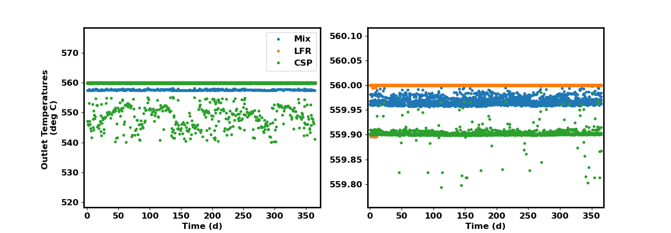
The hot outlet temperature for the mixed stream is the second largest, real eigenvalue if the eigenvalues are ordered from largest to smallest:

\[T_{mix}^H = \text{Re}\big\{\lambda^{\downarrow}_{2}(\mathbb{M})\big\}.\]

The final temperature solutions are shown below in a split-view figure (different zooms).

Mass Flow-Averaged Mixing

The above method was a rigorous way to solve for the mixed outlet temperature from both the nuclear and collector-receiver. An easier way to calculate the final temperature of the mixed streams would be to use a mass flow-average of the outlet temperatures.

The rationale behind this is that although the full specific heat formula is a cubic function of temperature, in the temperature domain we care about \(T \in [290^\circ C, 600^\circ C]\), the specific heat is linear and could be approximated to be constant.

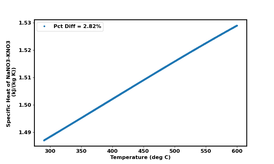
The figure shows specific heat plotted over the desired temperature domain as well as the percent difference in specific heat over the temperature domain. With a \(~ 2.8 \%\) difference in specific heat, we can approximate the specific heat as constant. We can extract the average specific heat as

\[\bar{C_p} = C_p(T_{avg})\]

where

\[T_{avg} = \frac{1}{2}(T_{salt}^H+T_{salt}^C).\]

With the original definition of specific heat

\[C_p(T) = \frac{dh}{dT} \bigg|_{P=\text{constant}}\]

we find that

\[\Delta h_{plant} = \bar{C_p}(T_{salt}^H - T_{salt}^C) = \bar{C_p} \Delta T_{salt}.\]

From the same enthalpy-mixing definition above

\[\Delta h_{mix} = \frac{\dot{m}_{nuc}^H \Delta h_{nuc} + \dot{m}_{rec}^H \Delta h_{rec}}{\dot{m}_{mix}^H} = \frac{\dot{m}_{nuc}^H\bar{C_p} \Delta T_{nuc} + \dot{m}_{rec}^H \bar{C_p} \Delta T_{rec}}{\dot{m}_{mix}^H}.\]

We then replace the left-hand side of the equation above with

\[\Delta h_{mix} = \bar{C_p} \Delta T_{mix}.\]

Combining the two equations, cancelling out specific heat, and assuming that the reference temperature in each \(\Delta T_{salt}\) is the same \(T_{salt}^C\) for each instance, we get

\[T_{mix}^H = \frac{\dot{m}_{nuc}^H T_{nuc}^H + \dot{m}_{rec}^H T_{rec}^H}{\dot{m}_{mix}^H}.\]

Plotting the difference between this mass flow-averaged and the previous enthalpy-averaged outlet temperatures for the mixed streams, we get the following figure:

Since the results are off on the order of milli-Kelvin, we can choose to use the mass flow-averaged solutions in the full implementation without loss in accuracy.